Explorative Analysis#
Uses the prostate time series dataset provided by the SurvSet package.
SurvSet package First install the dependencies:
%pip install 'njab[all]' openpyxl

import logging
Set parameters#
TARGET = "event"
TIME_KM = "time"
FOLDER = "prostate"
CLINIC = "https://raw.githubusercontent.com/RasmussenLab/njab/main/docs/tutorial/data/prostate/prostate.csv"
val_ids: str = ""  # List of comma separated values or filepath
#
# list or string of csv, eg. "var1,var2"
clinic_cont = ["age"]
# list or string of csv, eg. "var1,var2"
clinic_binary = ["male", "AD"]
# List of comma separated values or filepath
da_covar = "num_age,num_wt"
Time To Event: time
event (target) variable: event
Inspect the data:
| feat_name | event | time | fac_stage | fac_rx | fac_pf | fac_hx | fac_ekg | fac_bm | num_age | num_wt | num_sbp | num_dbp | num_hg | num_sz | num_sg | num_ap | num_sdate |
|---|---|---|---|---|---|---|---|---|---|---|---|---|---|---|---|---|---|
| pid | |||||||||||||||||
| 0 | 0 | 72 | 3 | 0.2 mg estrogen | normal activity | 0 | heart strain | 0 | 75 | 76 | 15 | 9 | 13.799 | 2 | 8 | 0.300 | 2,778 |
| 2 | 1 | 40 | 3 | 5.0 mg estrogen | normal activity | 1 | heart strain | 0 | 69 | 102 | 14 | 8 | 13.398 | 3 | 9 | 0.300 | 2,933 |
| 3 | 1 | 20 | 3 | 0.2 mg estrogen | in bed < 50% daytime | 1 | benign | 0 | 75 | 94 | 14 | 7 | 17.598 | 4 | 8 | 0.900 | 2,999 |
| 4 | 0 | 65 | 3 | placebo | normal activity | 0 | normal | 0 | 67 | 99 | 17 | 10 | 13.398 | 34 | 8 | 0.500 | 3,002 |
| 5 | 1 | 24 | 3 | 0.2 mg estrogen | normal activity | 0 | normal | 0 | 71 | 98 | 19 | 10 | 15.100 | 10 | 11 | 0.600 | 3,086 |
| ... | ... | ... | ... | ... | ... | ... | ... | ... | ... | ... | ... | ... | ... | ... | ... | ... | ... |
| 496 | 1 | 5 | 4 | 5.0 mg estrogen | normal activity | 1 | normal | 0 | 73 | 100 | 19 | 10 | 16.797 | 2 | 11 | 2.900 | 3,433 |
| 497 | 1 | 0 | 3 | 1.0 mg estrogen | normal activity | 0 | normal | 0 | 78 | 108 | 11 | 6 | 15.799 | 9 | 13 | 0.600 | 3,297 |
| 498 | 1 | 41 | 3 | 0.2 mg estrogen | normal activity | 1 | heart strain | 0 | 78 | 127 | 16 | 10 | 15.799 | 5 | 9 | 0.500 | 3,349 |
| 499 | 0 | 53 | 3 | 1.0 mg estrogen | normal activity | 0 | heart block or conduction def | 0 | 77 | 93 | 17 | 10 | 16.000 | 11 | 9 | 0.800 | 3,357 |
| 500 | 1 | 19 | 4 | 5.0 mg estrogen | normal activity | 1 | heart strain | 0 | 82 | 96 | 12 | 6 | 12.398 | 32 | 13 | 8.398 | 3,311 |
475 rows × 17 columns
Descriptive statistics of non-numeric variables:
clinic.describe(include="object")
| feat_name | fac_rx | fac_pf | fac_ekg |
|---|---|---|---|
| count | 475 | 475 | 475 |
| unique | 4 | 4 | 7 |
| top | 5.0 mg estrogen | normal activity | normal |
| freq | 121 | 428 | 161 |
Set the binary variables and convert them to categories:
vars_binary = ["fac_hx", "fac_bm"]
clinic[vars_binary] = clinic[vars_binary].astype("category")
Covariates to adjust for:
['num_age', 'num_wt']
Set continous variables
vars_cont = [
    "num_age",
    "num_wt",
    "num_sbp",
    "num_dbp",
    "num_hg",
    "num_sz",
    "num_sg",
    "num_ap",
    "num_sdate",
    "fac_stage",
]
Collect outputs#
in an excel file:
Output will be written to: prostate/1_differential_analysis.xlsx
Differences between groups defined by target#
Perform an uncontrolled t-test for continous and binomal test for binary variables. Besides the test results, summary statistics of both groups are provided.
First, set the binary target as a boolean mask:
happend = clinic[TARGET].astype(bool)
Univariate t-test for continous variables#
| event | no event | ttest | |||||||
|---|---|---|---|---|---|---|---|---|---|
| count | mean | std | count | mean | std | alternative | p-val | cohen-d | |
| variable | |||||||||
| num_sz | 338.000 | 15.660 | 13.071 | 137.000 | 10.898 | 9.066 | two-sided | 0.000 | 0.395 |
| num_sg | 338.000 | 10.506 | 2.034 | 137.000 | 9.796 | 1.899 | two-sided | 0.000 | 0.356 |
| num_hg | 338.000 | 13.255 | 2.027 | 137.000 | 13.825 | 1.638 | two-sided | 0.002 | 0.297 |
| num_age | 338.000 | 72.080 | 6.956 | 137.000 | 70.263 | 6.682 | two-sided | 0.008 | 0.264 |
| fac_stage | 338.000 | 3.462 | 0.499 | 137.000 | 3.336 | 0.474 | two-sided | 0.010 | 0.256 |
| num_wt | 338.000 | 98.107 | 13.735 | 137.000 | 101.255 | 12.073 | two-sided | 0.014 | 0.237 |
| num_sdate | 338.000 | 3,028.766 | 215.335 | 137.000 | 3,075.511 | 235.183 | two-sided | 0.046 | 0.211 |
| num_sbp | 338.000 | 14.426 | 2.398 | 137.000 | 14.255 | 2.515 | two-sided | 0.498 | 0.070 |
| num_dbp | 338.000 | 8.136 | 1.410 | 137.000 | 8.212 | 1.602 | two-sided | 0.630 | 0.052 |
| num_ap | 338.000 | 13.207 | 64.096 | 137.000 | 11.007 | 63.434 | two-sided | 0.733 | 0.034 |
Binomal test for binary variables:#
| event | no-event | binomial test | ||||||||
|---|---|---|---|---|---|---|---|---|---|---|
| count | p | count | p | k | n | alternative | statistic | pvalue | proportion_estimate | |
| variable | ||||||||||
| fac_hx | 338.000 | 0.500 | 137.000 | 0.277 | 169 | 338 | two-sided | 0.500 | 0.000 | 0.500 |
| fac_bm | 338.000 | 0.198 | 137.000 | 0.073 | 67 | 338 | two-sided | 0.198 | 0.000 | 0.198 |
Analaysis of covariance (ANCOVA)#
Next, we select continous variables controlling for covariates.
First the summary statistics for the target and covariates:
| feat_name | event | num_age | num_wt |
|---|---|---|---|
| count | 475.000 | 475.000 | 475.000 |
| mean | 0.712 | 71.556 | 99.015 |
| std | 0.454 | 6.920 | 13.341 |
| min | 0.000 | 48.000 | 69.000 |
| 25% | 0.000 | 70.000 | 90.000 |
| 50% | 1.000 | 73.000 | 98.000 |
| 75% | 1.000 | 76.000 | 107.000 |
| max | 1.000 | 89.000 | 152.000 |
Discard all rows with a missing features (if present):
| feat_name | event | num_age | num_wt |
|---|---|---|---|
| count | 475.000 | 475.000 | 475.000 |
| mean | 0.712 | 71.556 | 99.015 |
| std | 0.454 | 6.920 | 13.341 |
| min | 0.000 | 48.000 | 69.000 |
| 25% | 0.000 | 70.000 | 90.000 |
| 50% | 1.000 | 73.000 | 98.000 |
| 75% | 1.000 | 76.000 | 107.000 |
| max | 1.000 | 89.000 | 152.000 |
Remove non-varying variables (if present):
Run ANCOVA:
| test | ancova | |||||
|---|---|---|---|---|---|---|
| var | p-unc | np2 | -Log10 pvalue | qvalue | rejected | |
| feat_name | Source | |||||
| num_sz | event | 0.000 | 0.030 | 3.802 | 0.001 | True |
| num_sg | event | 0.000 | 0.025 | 3.304 | 0.002 | True |
| fac_stage | event | 0.013 | 0.013 | 1.883 | 0.035 | True |
| num_sdate | event | 0.024 | 0.011 | 1.621 | 0.039 | True |
| num_hg | event | 0.025 | 0.011 | 1.608 | 0.039 | True |
| num_sbp | event | 0.356 | 0.002 | 0.448 | 0.475 | False |
| num_ap | event | 0.721 | 0.000 | 0.142 | 0.824 | False |
| num_dbp | event | 0.873 | 0.000 | 0.059 | 0.873 | False |
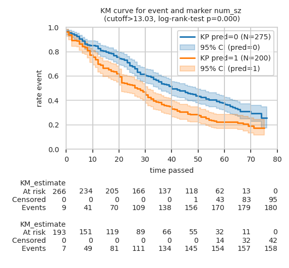
Kaplan-Meier (KM) plot for top markers#
Cutoff is defined using a univariate logistic regression
the default cutoff p=0.5 corresponds to a feature value of:
Optional: The cutoff could be adapted to the prevalence of the target.
List of markers with significant difference between groups as defined by ANCOVA:
| test | ancova | |||||
|---|---|---|---|---|---|---|
| var | p-unc | np2 | -Log10 pvalue | qvalue | rejected | |
| feat_name | Source | |||||
| num_sz | event | 0.000 | 0.030 | 3.802 | 0.001 | True |
| num_sg | event | 0.000 | 0.025 | 3.304 | 0.002 | True |
| fac_stage | event | 0.013 | 0.013 | 1.883 | 0.035 | True |
| num_sdate | event | 0.024 | 0.011 | 1.621 | 0.039 | True |
| num_hg | event | 0.025 | 0.011 | 1.608 | 0.039 | True |
Settings for plots
class_weight = "balanced"
y_km = clinic[TARGET]
time_km = clinic[TIME_KM]
compare_km_curves = partial(
    compare_km_curves,
    time=time_km,
    y=y_km,
    xlim=(0, 80),
    xlabel="time passed",
    ylabel=f"rate {y_km.name}",
)
log_rank_test = partial(
    log_rank_test,
    time=time_km,
    y=y_km,
)
TOP_N = 2  # None = all
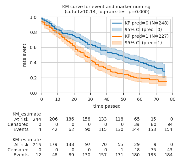
Plot KM curves for TOP_N (here two) makers with log-rank test p-value:
Intercept -0.512, coef.: 0.039
/usr/bin/sh: 1: Syntax error: "(" unexpected
Custom cutoff defined by Logistic regressor for     num_sz: 13.031
Intercept -1.862, coef.: 0.184
/usr/bin/sh: 1: Syntax error: "(" unexpected
Custom cutoff defined by Logistic regressor for     num_sg: 10.142